Lure point transect case study: Scottish crossbills
The Scottish crossbill is Britain’s only endemic bird species. A lure point transect survey was used to estimate its population size (Summers and Buckland 2011). In this case study, we work through the analyses reported in Section 10.2.1 of the book. We do not attempt to recreate those analyses exactly; instead, we simplify the analyses, while retaining the essential elements to allow the approach to be adapted to other studies.
1 The trials
The trials data are in file lure trials.csv. We first read the data:
xbill <- read.table("lure trials.csv", header = T, sep = ",")
attach(xbill)
We next specify a distance (in metres) beyond which it is reasonable to assume that no crossbill will respond to the lure:
w <- 850There are several covariates in the data that might affect probability that a bird responds to the lure: day (days from 1st January); time (hour of the day); habitat (1 = plantation, 2 = native pinewood); behavcode (1 = perching and feeding, 2 = giving excitement calls, 3 = singing); numbirds (flock size); and dist (distance of birds from the point when the lure was played). We can fit all these covariates as follows.
habitat <- factor(habitat)
behavcode <- factor(behavcode)
model1 <- glm(response ~ dist + numbirds + day + time + habitat + behavcode,
    family = binomial)
summary(model1)
Call:
glm(formula = response ~ dist + numbirds + day + time + habitat +
    behavcode, family = binomial)

Deviance Residuals:
    Min       1Q   Median       3Q      Max
-1.9526  -0.8708   0.5563   0.8168   2.0009

Coefficients:
             Estimate Std. Error z value Pr(>|z|)
(Intercept)  2.641601   1.301148   2.030   0.0423 *
dist        -0.010086   0.002323  -4.342 1.41e-05 ***
numbirds     0.076882   0.081172   0.947   0.3436
day         -0.008597   0.007405  -1.161   0.2456
time        -0.020251   0.113258  -0.179   0.8581
habitat2    -0.263713   0.574532  -0.459   0.6462
behavcode2   0.070903   0.495256   0.143   0.8862
behavcode3   0.962426   0.614541   1.566   0.1173
---
Signif. codes:  0 '***' 0.001 '**' 0.01 '*' 0.05 '.' 0.1 ' ' 1

(Dispersion parameter for binomial family taken to be 1)

    Null deviance: 219.23  on 166  degrees of freedom
Residual deviance: 169.10  on 159  degrees of freedom
  (8 observations deleted due to missingness)
AIC: 185.1

Number of Fisher Scoring iterations: 5anova(model1)Analysis of Deviance Table
Model: binomial, link: logit
Response: response
Terms added sequentially (first to last)
Df Deviance Resid. Df Resid. Dev
NULL 166 219.23
dist 1 44.961 165 174.27
numbirds 1 1.514 164 172.76
day 1 0.825 163 171.93
time 1 0.115 162 171.82
habitat 1 0.022 161 171.80
behavcode 2 2.694 159 169.10We see that only dist has a coefficient that is significantly different from zero. Experiment with dropping non-significant terms. Using a backwards stepping procedure, you should find that other covariates remain non-significant, so we can use the simple model:
model2 <- glm(response ~ dist, family = binomial)
summary(model2)
Call:
glm(formula = response ~ dist, family = binomial)

Deviance Residuals:
    Min       1Q   Median       3Q      Max
-1.9521  -0.8066   0.5957   0.7618   1.9355

Coefficients:
            Estimate Std. Error z value Pr(>|z|)
(Intercept)  2.16370    0.33944   6.374 1.84e-10 ***
dist        -0.01049    0.00210  -4.993 5.94e-07 ***
---
Signif. codes:  0 '***' 0.001 '**' 0.01 '*' 0.05 '.' 0.1 ' ' 1

(Dispersion parameter for binomial family taken to be 1)

    Null deviance: 227.52  on 174  degrees of freedom
Residual deviance: 179.44  on 173  degrees of freedom
AIC: 183.44

Number of Fisher Scoring iterations: 5
(Degrees of freedom change a little as some covariates have a few missing values.)
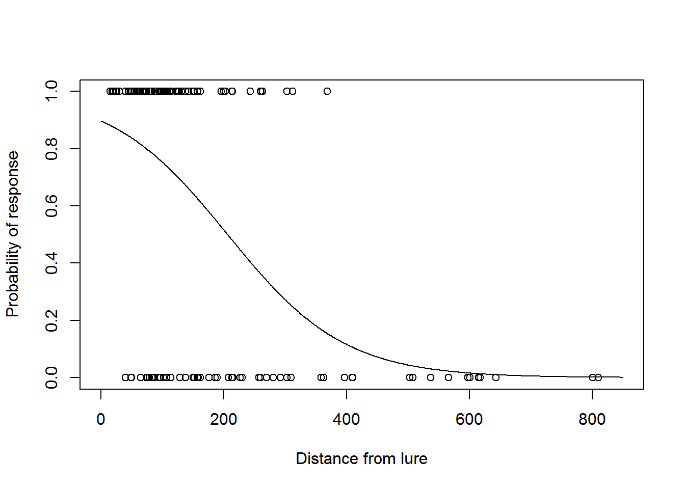
We can now plot the fitted detection function model:
fits <- fitted(model2)
plot(dist, response, xlim = c(0, w), xlab = "Distance from lure", ylab = "Probability of response")
dist2 <- 0:w
phat <- predict.glm(model2, newdata = data.frame(dist = dist2), type = "response")
lines(dist2, phat)
2 The survey
We need to specify the function /pi(r),r/lew/pi(r),r/lew, which represents the probability density function of distances of animals from the point. If we extend the study area out a distance w around the entire boundary, thus creating a bufferzone, and place our survey points at random throughout the area + bufferzone (or randomly place a systematic grid of points over the extended study area), we can assume that this density is triangular:
pi_r <- dist2/sum(dist2)If the study area is fragmented, it may not be cost-effective to sample into the bufferzone. If points are restricted to within the boundaries of the study area, and the species of interest does not occur beyond the study area because habitat is unsuitable, we need to adjust /pi(r)/pi(r) so that it reflects the amount of available habitat (averaged over points) with increasing distance from the point (Buckland et al. 2006). (Summers and Buckland 2011) estimated this availability function, but for the purposes of this case study, we use the above triangular distribution.
# Pa is prob of response, integrating r from 0 to w, assuming that phat is a
# function of distance alone (no z's in model)

(Pa <- sum(phat * pi_r))
[1] 0.09709381Thus we estimate that just under 10% of birds within 850m of a point are detected. We now read in the data from the main survey. Note that detection distances are unknown in the main survey; instead, we have used the trials data to estimate the detection function, and hence the proportion of birds within 850m that are detected.
detections <- read.table("mainsurveydetections.csv", sep = ",", header = T)
attach(detections)
We now calculate the number of points kmain in the main survey, and the total area a within 850m of a point, converting from m2 to km2. (Note that, if we do not include unsuitable habitat as described above, this total area should also exclude that habitat.)
kmain <- length(point)
a <- kmain * pi * (w/1000)^2
A <- 3505.8  # size in km2 of study area
We can now estimate the size of the population as
(Nscot <- sum(nscottish) * A/(Pa * a))[1] 10007.67Thus we estimate that there are around 10,000 birds. (This does not agree with the estimate of 13,600 in (Summers and Buckland 2011), because we have opted to keep the case study simple, and have omitted corrections for unsuitable habitat on surveyed plots, for juveniles, for unidentified crossbills, for incubating or brooding females, and for flying birds. Correcting only for unsuitable habitat on surveyed plots increases the abundance estimate to 12,900 birds.)
3 Measure of precision
We can calculate a standard error for our estimate and a 95% confidence interval for true abundance by bootstrapping both trials and points:
index <- 1:kmain
nboot <- 999
bNscot <- vector(length = nboot)
m <- length(dist)
tindex <- 1:m
bdist <- vector(length = m)
bresponse <- vector(length = m)
for (i in 1:nboot) {
    # bootstrap trials
    btindex <- sample(tindex, m, replace = TRUE)
    for (l in tindex) {
        bdist[l] <- dist[btindex[l]]
        bresponse[l] <- response[btindex[l]]
    }
    bmodel <- glm(bresponse ~ bdist, family = binomial)
    bphat <- predict.glm(bmodel, newdata = data.frame(bdist = dist2), type = "response")
    bPa <- sum(bphat * pi_r)
    # bootstrap points
    rindex <- sample(index, kmain, replace = TRUE)
    bNscot[i] <- sum(nscottish[rindex]) * A/(bPa * a)
}
# calculate bootstrap standard error
seNscot <- sd(bNscot)
# calculate bootstrap percentile confidence limits
bNscot <- sort(bNscot)
alpha.over.2 <- 0.025
loNscot <- bNscot[round(alpha.over.2 * (nboot + 1))]
hiNscot <- bNscot[round((1 - alpha.over.2) * (nboot + 1))]
(c(Nscot, seNscot, loNscot, hiNscot))
[1] 10007.672 3058.370 5789.635 17980.691Thus we estimate the population size to be 10008 birds with standard error 3058 and 95% confidence interval (5790, 17981).
References
Buckland, S. T., R. W. Summers, D. L. Borchers, and L. Thomas. 2006. Point transect sampling with traps or lures. Journal of Applied Ecology 43:377—384.
Summers, R. W., and S. T. Buckland. 2011. A first survey of the global population size and distribution of the Scottish Crossbill loxia scotica. Bird Conservation International 21:186—198.