Covariates in detectability case study, Hawaiian amakihi
This case study is intended to duplicate the findings shown in Section 5.3.2 of the book which duplicates the analysis presented by Marques et al. (2007). This document describes the analysis of these data both using the Distance GUI software as well as analysis in R.
1 Amakihi analysis using the Distance software
This set of data is included in the distribution of Distance as one of the Sample Projects. You can open this project (entitled amakihi.zip) in the Sample project directory underneath My Distance projects directory residing under My Documents. Open and extract the contents of the archived .zip file to any convenient location on your computer.
1.1 Data summary
When the project is unzipped and opens, have a brief look at the nature of the data using the Data tab. You will see fields corresponding to the description in Section 5.3.2.1. Specifically, check that the Point labels run from 1 to 41, representing the 41 point transects sampled. You can see from the observation ID column there are 1434 sighting in this dataset (not the 1485 noted in Section 5.3.2.1). Finally looking at the Region ID field you will find there are 7 “regions” corresponding to the 7 replicate surveys conducted that are represented in this project as temporal strata. Consequently the data are sorted by transect within region. Points are visited an equal number of times during each survey period, so the amount of survey effort is “1” for all points.
1.2 Analysis summary
Moving to the Analysis tab, you will find a set of 16 model definitions in the Project browser. These are the models described in Table 2 of Marques et al. (2007). Table 5.7 of Distance sampling: Methods and applications does not discuss models with survey-specific detection functions. Note all of the models in the project have the same data filter applied to them; the filter truncates detections at 82.5m.
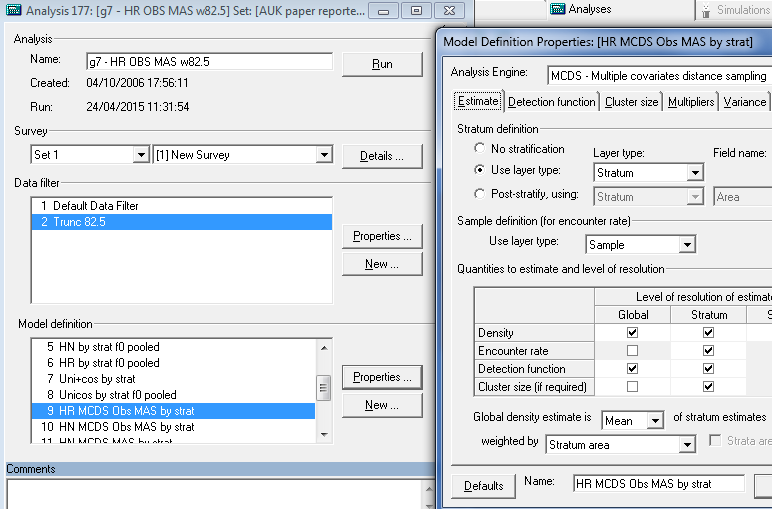
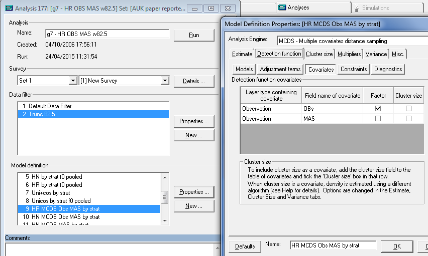
Drawing attention to the model named j10 - HN OBS MAS w82.5, this is the model chosen by AIC as the preferrable model for this data set. The screen captures below show a) the appropriate checkboxes to have a common detection function across all strata and b) choosing the covariates for the model and treating observer as a factor covariate.
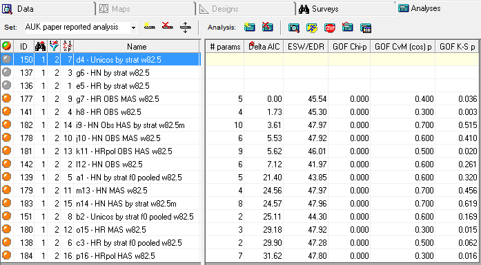
All models can be fitted concurrently by highlighting multiple rows in the Project Browser and choosing the running man icon (fourth from right). With all 13 models from Table 5.7 of the book fitted (and a few extra thrown in), you can nearly duplicate Table 5.7.
By employing the final icon to the right in the Analysis tab menu, you can alter the columns that appear in the Results Browser to include/exclude results. Clicking on the header of any column in the results browser (such as Delta AIC) will sort the table on that column. The resulting table (below) matches the values shown in Table 5.7.
2 Amakihi analysis in R
Analysis begins by acquiring the data from a comma-delimited file (this file was created by copying the data from the amakihi Distance project and removing a few columns.)
library(Distance)
amakihi <- read.csv(file="amakihi.csv")
scalemin <- sd(amakihi$MAS, na.rm = TRUE) # used in plotting
2.1 Exploratory data analysis
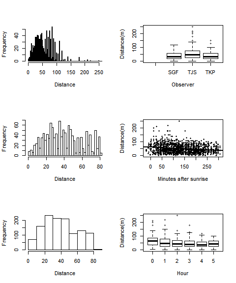
As discussed in Section 5.3.2.1, “it is important to gain an understanding of the data prior to fitting detection functions”. With this in mind, preliminary analysis of distance sampling data involves
- assess the shape of the collected data,
- consider the level of truncation of detections, and
- explore patterns in potential covariates
par(mfrow=c(3,2))
hist(amakihi$distance, breaks=seq(0,260), main="",xlab = "Distance")
boxplot(amakihi$distance[!amakihi$OBS==""]~amakihi$OBS[!amakihi$OBS==""],
        xlab="Observer", ylab="Distance(m)")
hist(amakihi$distance[amakihi$distance<82.5], breaks=33,
     main="",xlab = "Distance")
plot(amakihi$MAS, amakihi$distance,
     xlab="Minutes after sunrise", ylab="Distance(m)",
     pch=19, cex=0.6)
abline(reg=lm(amakihi$distance~amakihi$MAS),lwd=2)
hist(amakihi$distance[amakihi$distance<82.5], breaks=10,
     main="",xlab = "Distance")
boxplot(amakihi$distance~amakihi$HAS,
        xlab="Hour", ylab="Distance(m)")
par(mfrow=c(1,1))2.2 Adjusting the raw covariates
Two adjustments need to be made to the covariates prior to analysis. Recall in the Distance project above, the Factor box was checked for the covariate OBS to indicate that the observer covariate was to be treated as a factor variable. When performing the analysis in R, you will note that OBS was read in as a factor variable because it consisted of characters
str(amakihi$OBS)## Factor w/ 4 levels "","SGF","TJS",..: 3 3 3 3 3 3 3 3 3 3 ...however because HAS (hours after sunrise) was a numeric variable, it was read in as an integer. That is fine if we wish to include HAS in our model with the effect of HAS being monotonic (i.e., detectability either steadily increases or steadily decreases as a function of HAS). If we wish to allow HAS to have a non-linear effect on detectability, then we convert the integer HAS to a factor (this is how HAS was treated in the original analysis; have a look at model definition HN MCDS Obs HAS by strat in the Distance project).
amakihi$HAS <- as.factor(amakihi$HAS)
amakihi$OBS <- relevel(amakihi$OBS, ref="TKP")
amakihi$HAS <- relevel(amakihi$HAS, ref="5")
The final adjustment shown above, is to change the reference level of the observer and hour factor covariates. The only reason we use the relevel() function here is to get the estimated parameters in the detection function to match the parameters estimated by Distance.
More subtle is a transformation of the continuous covariate, MAS (minutes since sunrise). We are entertaining three possible covariates in our detection function: observer, hours and minutes since sunrise. Observer and hours are both factor variables, that we can think of as taking on values between 1 and 3 in the case of observer, and 1 to 6 in the case of hours. However minutes can take on values from -9 (detections before sunrise) to >300. The disparity in scales of measure between MAS and the other candidate covariates can lead to difficulties in the performance of the optimiser fitting the detection functions in R. The solution to the difficulty is to scale MAS such that is on a scale (~1 to 5) comparable with the other covariates.
Dividing all the MAS measurements by the standard deviation of those measurements accomplishes the desired compaction of the range of the MAS covariate without changing the shape of the distribution of MASvalues.
amakihi$MAS <- amakihi$MAS/sd(amakihi$MAS, na.rm=TRUE)2.3 Detection function fitting and goodness of fit
The Distance package in R can fit all of the models presented in Table 5.7 of the book. The function ds()performs the detection function fitting and in the mrds package, there is a function ddf.gof() that performs goodness of fit tests (in the form of /chi2/chi2, Cramer von Mises and Kolomogorov-Smirnov tests).
2.3.1 Helper function
I built a convenient wrapper function to combine calls to both ds() and ddf.gof() in the same function. Motivation for this was to be able to duplicate Table 5.7 of the book.
fit.and.assess <- function(data=amakihi, key="hn",
                           adj="cos", order=NULL,
                           cov=c("MAS"), truncation=82.5,
                           plotddf = FALSE, ...) {
#  wrapper function to combine detection function fitting as well as
#  goodness of fit testing into a single function
#
#  Input - name of dataframe, key/adjustment combination, order of adjustment terms,
#          and a vector of covariates to include in detection function
#          specifically for this example, I limit number of covariates to 2,
#          truncation distance (default value for amakihi),
#          flag plotddf to signal whether a plot of the detfn is required
#
#  Output - named list containing the columns of Table 5.7 (with the exception
#           of the effective detection radius).  List will subsequently be
#           post-processed to duplicate the table.

  if (length(cov)>2) stop("Function can take no more than 2 covariates")
  mystring <- ifelse(length(cov)==2,
                     paste(cov[1],cov[2],sep="+"),
                     cov[1])
  covariates <- as.formula(paste("~", mystring))
  model.fit <- ds(data, key=key, adjustment=adj,
                  formula=covariates, transect="point", order=order,
                  truncation = truncation)
  if (plotddf) plot(model.fit, pl.den=0, pch=19,
                    cex=0.7, main=paste(key, adj, cov))
  aic <- model.fit$ddf$criterion
  pars <- length(model.fit$ddf$par)
  gof <- ddf.gof(model.fit$ddf)
  chisq.p <- gof$chisquare$chi1$p
  cvm.p <- gof$dsgof$CvM$p
  ks.p <- gof$dsgof$ks$p
  findings <- list(formula=mystring, key=key, aic=aic, pars=pars,
                   chisq.p=chisq.p, cvm.p=cvm.p, ks.p=ks.p)
  return(findings)
}
2.3.2 Candidate models
It is not best practice to take a scattergun approach to detection function model fitting, but the candidate model set is presented in Table 5.7 of the book, the straightforward way to fit the 13 models is to make 13 calls to the helper function just described:
hour.hn <- fit.and.assess(key="hn", order=2, cov=c("HAS"))
hour.hr <- fit.and.assess(key="hr", adj=NULL, cov=c("HAS"))
obs.hour.hn <- fit.and.assess(key="hn", order=0, cov=c("OBS","HAS")) # fails if order>0
obs.hour.hr <- fit.and.assess(key="hr", adj=NULL, cov=c("OBS","HAS"))
obs.min.hn <- fit.and.assess(key="hn",order=0, cov=c("OBS","MAS")) # fails if order>0
obs.min.hr <- fit.and.assess(key="hr", adj=NULL, cov=c("OBS","MAS"))
min.hn <- fit.and.assess(key="hn", order=0, cov=c("MAS")) # fails if order>0
min.hr <- fit.and.assess(key="hr", adj=NULL, cov=c("MAS"))
obs.hn <- fit.and.assess(key="hn", order=0, cov=c("OBS")) # fails if order>0
obs.hr <- fit.and.assess(key="hr", adj=NULL, cov=c("OBS"))
hn <- fit.and.assess(key="hn",  order=(2:5), cov=c(1))
hr <- fit.and.assess(key="hr", adj=NULL, cov=c(1))
uni <- fit.and.assess(key="uni", cov=c(1))
Note the use of the cov=c(1) notation to choose to fit a model with no covariates.
2.3.3 Summarise model selection
We gather results of 13 model fits into a single data frame, using a function found in the data.table package to bind together lists into rows of a dataframe.
library(data.table)
library(knitr)
mymodels <- list(hour.hn, hour.hr, obs.hour.hn, obs.hour.hr,
                 obs.min.hn, obs.min.hr, min.hn, min.hr,
                 obs.hn, obs.hr, hn, hr, uni)
results.frame<- rbindlist(mymodels)
results.frame <- results.frame[order(results.frame$aic), ] #   sort by increasing AIC
smallest <- results.frame[1, aic]  # note syntax for data.table
results.frame$deltaaic <- results.frame$aic - smallest
setcolorder(results.frame, c("formula","key","pars","deltaaic","chisq.p","cvm.p","ks.p","aic"))
kable(results.frame[,.(formula, key, pars, deltaaic, chisq.p, cvm.p, ks.p)], digits=c(0,0,0,1,0,3,3), caption="Attempt to duplicate Table 5.7 using R function `ds` from the Distance package.")| formula | key | pars | deltaaic | chisq.p | cvm.p | ks.p |
|---|---|---|---|---|---|---|
| OBS+MAS | hr | 5 | 0.0 | 0 | 0.389 | 0.076 |
| OBS | hr | 4 | 1.1 | 0 | 0.271 | 0.025 |
| OBS+HAS | hr | 9 | 5.8 | 0 | 0.450 | 0.084 |
| 1 | hn | 5 | 21.7 | 0 | 0.557 | 0.338 |
| OBS+HAS | hn | 8 | 23.7 | 0 | 0.011 | 0.028 |
| 1 | uni | 2 | 25.4 | 0 | 0.440 | 0.169 |
| OBS+MAS | hn | 4 | 26.5 | 0 | 0.008 | 0.025 |
| MAS | hr | 3 | 28.3 | 0 | 0.558 | 0.257 |
| 1 | hr | 2 | 30.2 | 0 | 0.334 | 0.063 |
| HAS | hr | 7 | 30.8 | 0 | 0.580 | 0.289 |
| HAS | hn | 7 | 35.5 | 0 | 0.228 | 0.164 |
| OBS | hn | 3 | 39.1 | 0 | 0.003 | 0.001 |
| MAS | hn | 2 | 49.2 | 0 | 0.007 | 0.020 |
Duplication of Table 5.7 is not exact. The main discrepency lies in that the R function ds() has convergence challenges with adjustment terms and covariates in detection functions. That is not a problem for the amakihi hazard rate key function models (they did not use adjustment terms). But the half-normal key functions employed adjustment terms in the original Marques et al. (2007) analysis. Models OBS+HAS, OBS+MAS, OBSand MAS with a half-normal key function all failed to converge, so they were fitted without adjustment terms. In each model, the model without adjustments had AIC scores >20 AIC units larger than the same models that included adjustments (fitted in Distance for Windows). As a consequence, models that should have had adjustment terms are models with the two largest AICs, while OBS+HAS should have AIC values of 3.6 rather than 23.7 and OBS+MAS should have AIC values of 5.5 rather than 26.5; if a more robust optimisation engine were available in R. Note also that the Cramér von Mises goodness of fit P-value is very small for the models fitted without adjustment terms.
2.3.4 Inference from best model
The model with the lowest AIC used the hr key function with covariates OBS+MAS. The shape of the detection function is
bestmod <- ds(amakihi,trunc=82.5,key="hr",adj=NULL,formula=~OBS+MAS)
pred.haz.obs.minute <- function(pars, trunc=82.5, obs2=0, obs3=0, mas=0) {
#   creates hazard rate detection function for plotting
#   based upon parameters of detection function and covariate values
#   tailored for the OBS+MAS covariate model
  distances <- seq(0, trunc, length=100)
  nu <- pars[2] + pars[3]*obs2 + pars[4]*obs3 + pars[5]*mas
  sigma <- exp(nu)
  mycurve <- (1-exp(-(distances/sigma)^-pars[1])) # / (1-exp(0^-pars[1]))
  return(mycurve)
}
par(mfrow=c(1,2))
dists <- seq(0, 82.5, length.out = 100)
obs1.min0 <- pred.haz.obs.minute(bestmod$ddf$par)
obs2.min0 <- pred.haz.obs.minute(bestmod$ddf$par, obs2=1)
obs3.min0 <- pred.haz.obs.minute(bestmod$ddf$par, obs3=1)
plot(dists, obs1.min0, type='l', ylim=c(0,1),
     ylab="Detection probability by OBS", xlab="Distance (m)")
lines(dists, obs2.min0, lty=2)
lines(dists, obs3.min0, lty=3)

obs1.0 <- pred.haz.obs.minute(bestmod$ddf$par)
obs1.60 <- pred.haz.obs.minute(bestmod$ddf$par,mas=60/scalemin)
obs1.120 <- pred.haz.obs.minute(bestmod$ddf$par,mas=120/scalemin)
obs1.180 <- pred.haz.obs.minute(bestmod$ddf$par,mas=180/scalemin)
obs1.240 <- pred.haz.obs.minute(bestmod$ddf$par,mas=240/scalemin)

plot(dists, obs1.0, type='l', ylim=c(0,1),
     ylab="Detection probability by MAS", xlab="Distance (m)")
lines(dists, obs1.60)
lines(dists, obs1.120)
lines(dists, obs1.180)
lines(dists, obs1.240)
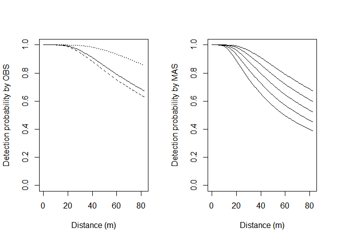
Hazard rate detection function plotted for three observers in the Amakihi study (left) and for Observer1 and sunrise, 1, 2, 3 and 4 hours after sunrise. Based on model with OBS+MAS as covariates.
par(mfrow=c(1,1))References
Marques, T. A., L. Thomas, S. G. Fancy, and S. T. Buckland. 2007. Improving estimates of bird density using multiple covariate distance sampling. The Auk 124:1229–1243.